[ML] 10. EM Algorithm

Intro

주어지는 data에 항상 feature, label이 정확하게 매칭되지는 않는다. 이럴 경우 우리는 각 data에 대한 label과 주어진 data와 label을 잘 설명할 수 있는 probability distribution을 모두 구해야 한다. 여기서 label과 probability distribution을 동시에 구하기 위해서는 어떻게 해야할지에 대한 방법 중에서 대표적인 EM Algorithm에 대해서 살펴보도록 하겠다.

Problem

여태까지 우리가 살펴봤던 supervised learning에서는 학습(learning) 시에는 feature와 label이 모두 동시에 주어지고, 예측/추론(inference)을 수행할 때에는 feature만 존재하는 data가 주어졌다. 따라서, 학습 시에 feature 정보들을 특정 pattern에 녹여냈을 때, label값을 얻는지를 확인할 수 있었다. 하지만, label이 주어지지 않은 data를 학습시킬 때에는 어떻게 해야할까? 우리는 label이 있어야 해당 data가 가진 실제 결과값을 알고 probability distribution을 얼마나 수정할지를 알 수 있었다. 하지만, 이 값을 모르니 probability distribution을 만들 수 없다. 정확한 probability distribution이 있다면, 반대로 label을 생성하는 것도 가능할 것이다. 하지만, 우리는 아무것도 알 수 없다.

이렇게 답답한 상황에서 우리는 다음과 같은 아이디어를 발상해낼 수 있다. 만약, 대략적인 label을 안다면, 이것을 이용해서 최적의 확률 분포를 찾고, 이 확률 분포에 맞는 label을 다시 생성하고 이를 기반으로 다시 확률 분포를 찾는다면 어떨까? 이렇게 반복하면 꽤나 그럴싸한 분포를 만들 수 있지 않을까? 이 과정을 예를 들자면, 다음과 같다.

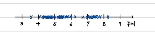
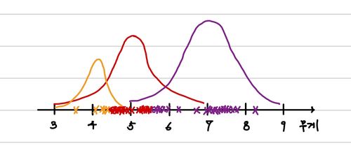
각 기 다른 나라(label)의 동전 3종류(500원, 100cent, 100엔)를 구분하고 싶다고 하자. 이때, 알 수 있는 정보는 무게(feature) 밖에 없다고 가정하겠다. 이때 우리는 어떻게 구분할 수 있을까? 우리가 길 거리에서 무작위로 동전을 수집했다고 하자. 각 동전은 흠집도 있을 것이고 공장마다 조금씩 무게가 차이있을 수 있다. 그 결과 다음과 같은 분포가 나왔다고 하자.

ml-em-algorithm-1

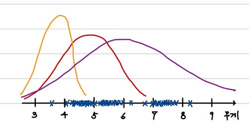
그래서 우리는 확률 분포가 아마 Gaussian distribution이라고 생각할 것이다. 따라서, 임의의 Gaussian Distribution을 따르는 세 개의 분포를 아래와 같이 가정해보는 것이다.

ml-em-algorithm-2

그렇다면, 우리는 이 분포에 따라 가장 적절한 label을 생성할 수 있다. 아래와 같이 생성할 수 있다.

ml-em-algorithm-3

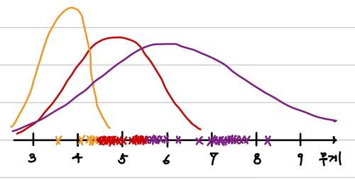
그러면 결과적으로 우리는 다음과 같은 label된 data를 갖게 되는 것이다.

ml-em-algorithm-4

이렇게 labeling data를 이용해서 우리는 더 효과적인 확률 분포 변수를 찾아보면 아래와 같이 이전과는 사뭇 다른 분포를 가진다는 것을 알 수 있다.

ml-em-algorithm-5

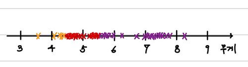
결과적으로 해당 분포가 이전에 임의로 추정했던 분포보다 더 적절하다는 것을 알 수 있다. 이 과정을 계속해서 반복하면 어떻게 될까?

ml-em-algorithm-6

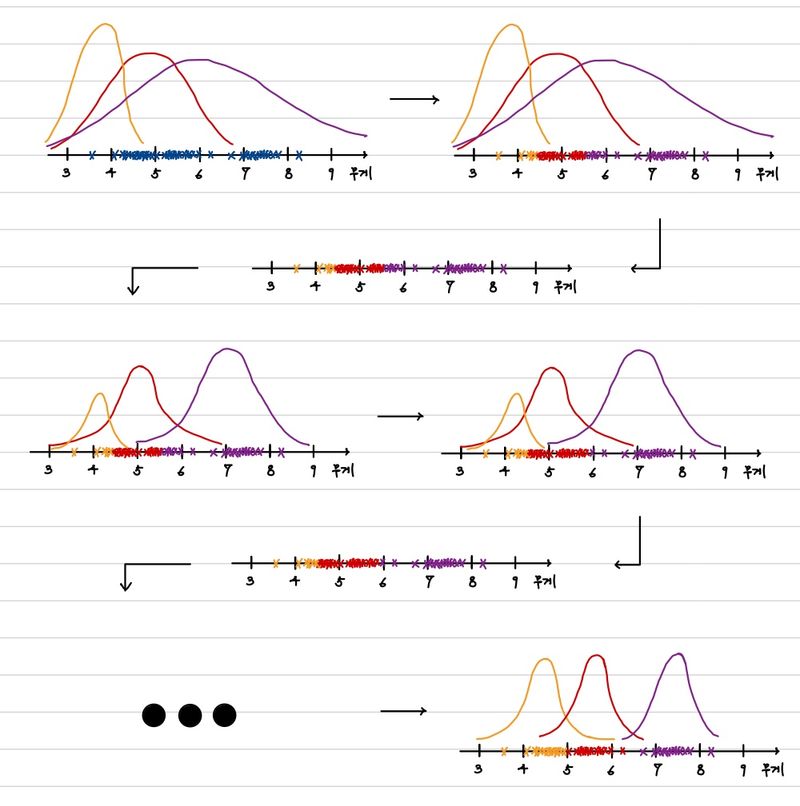
반복을 통해서 우리는 그럴싸한 확률분포를 습득했다. 대략 머릿속으로는 그럴 수 있을 것 같다는 생각이 들 것이다. 그렇다면, 이것이 어떻게 가능하며 수학적으로 표현이 가능할까? 이를 이제부터 자세히 알아보도록 하겠다.

Base Knowledge

본론으로 들어가기에 앞 서 우리는 두 가지 정의를 알아야 EM Algorithm을 증명하고 설명할 수 있다.

Jensen’s Inequality
Gibb's Inequality

이 두 가지를 모두 안다면 바로 다음으로 넘어가는 것이 좋다. 하지만, 알지 못한다면 이 정의에 대해서 먼저 알아보고 가도록 하자.

Jensen’s Inequality

일반적으로 우리는 다음 성질을 만족하는 집합을 Convex set이라고 한다.

\lambda x + (1-\lambda)y \in C,\quad \forall x, y \in C \text{ and } \forall\lambda\in[0,1]

즉, 집합에서 random으로 고른 두 수 사이의 수도 집합에 포함되는 집합이라는 것이다. convex set이라고 불리는 이유는 결국 이러한 집합을 2, 3 차원상에 그려보면 볼록하게 튀어나오는 형태라는 것을 알 수 있기 때문이다.

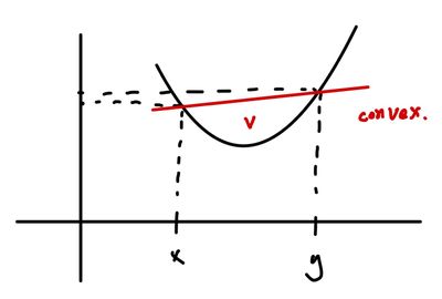
또한, 아래와 같은 조건을 만족하는 함수(f)를 Convex function이라고 한다.

f(\lambda x + (1-\lambda)y) \leq \lambda f(x) + (1-\lambda)f(y),\quad \forall x,y \in C(\text{Convex set}) \text{ and } \forall\lambda \in [0,1]

아래로 볼록한 함수에서는 위와 같은 과정이 너무나 당연하게도 성립한다. 사잇값의 함수값보다 함수값의 사잇값이 더 크기 때문이다.

ml-convex-function

반대로 concave(위로 볼록) 함수인 경우에는 반대로 다음과 같이 정의된다.

f(\lambda x + (1-\lambda)y) \geq \lambda f(x) + (1-\lambda)f(y),\quad \forall x,y \in C(\text{Convex set}) \text{ and } \forall\lambda \in [0,1]

여기서 Jensen's Inequality는 다음과 같은 수식이 convex에서 성립한다는 것이다.

E[f(X)] \geq f(E[X])

convex function에서는 어찌보면 당연해보인다. 그렇지만 이는 EM Algorithm에서 토대로 사용되는 아이디어이기 때문에 반드시 기억하자. 반대로 Concave function인 경우에는 다음과 같다.

E[f(X)] \leq f(E[X])

Gibb's Inequality

KL divergence 식에 Jensen's Inequality를 적용하여 KL divergence가 항상 0보다 크거나 같고, KL divergence가 0이 되기 위해서는 두 확률분포가 같아야 한다는 것을 증명한 것이다.

이에 대한 증명을 간단하게 하면 다음과 같다.

\begin{align*} KL(p||q) &= \sum_{i}{p_{i}\log\frac{p_{i}}{q_{i}}} \\ &= -\sum_{i}p_{i}\log{\frac{q_{i}}{p_{i}}} \\ &= E_{p}[-\log{\frac{q_{i}}{p_{i}}}] \geq -\log{E_{p}[\frac{q_{i}}{p_{i}}]}\, (\because \text{Jensen's Inequality}) \\ &= -\log{\sum_{i}p_{i}\frac{q_{i}}{p_{i}}} = -\log{1} = 0\\ \therefore KL(p||q) &\geq 0 \end{align*}

EM Algorithm

우리는 parametric estimation 방법을 사용하기 위해서 다음과 같은 Likelihood를 계산했다.

\begin{align*} \mathcal{L}(\theta) &= \log p(D| \theta) \\ \mathcal{L}(\theta) &= \log \prod_{x\in D} p(x| \theta) \\ &= \sum_{x\in D} \log{p(x|\theta)} \end{align*}

그렇지만 우리가 이 값을 구하는 것이 어렵다는 것을 위에서 제시했다. 따라서, 이를 다음과 같이 바꿔서 풀어보자는 것이다.

\begin{align*} \mathcal{L}(\theta) &= \sum_{x\in D} \log{p(x|\theta)} \\ &= \sum_{x\in D} \log{\int_{z \in K}p(x, z|\theta)} dz \end{align*}

이렇게 바꾸게 된다고 무슨 이득이 있을까? 단순히 식이 더 복잡해보인다. 하지만, 이 식을 다음과 같이 바꿀 수 있다.

\begin{align*} \mathcal{L}(\theta) &= \sum_{x\in D} \log{p(x|\theta)} \\ &= \sum_{x\in D} \log{\int_{z \in K} p(x, z|\theta)} dz \\ &= \sum_{x\in D} \log{\int_{z \in K} p(x, z|\theta) \frac{p(z|x, \theta^{\prime})}{p(z| x, \theta^{\prime})} dz} \\ &= \sum_{x\in D} \log{\int_{z \in K} p(z|x, \theta^{\prime}) \frac{p(x, z|\theta)}{p(z| x, \theta^{\prime})} dz} \\ &= \sum_{x\in D} \log{E_{z|x, \theta^{\prime}}{[\frac{p(x, z|\theta)}{p(z| x, \theta^{\prime})}]}} \geq \sum_{x\in D} E_{z|x, \theta^{\prime}}{[\log{\frac{p(x, z|\theta)}{p(z| x, \theta^{\prime})}}]}\,(\because \text{Jensen's Inequality}) = \mathcal{F}(p_{z|x, \theta^{\prime}}, \theta) \end{align*}

이를 통해서 우리는 아래와 같은 과정을 수행해볼 수 있다.

\begin{align*} \mathcal{L}(\theta) - \mathcal{F}(p_{z|x, \theta^{\prime}}, \theta) &= \sum_{x\in D} \log{p(x|\theta)} - \sum_{x\in D}\{\int_{z|x, \theta^{\prime}}{p(z|x,\theta^{\prime})\log{\frac{p(x, z|\theta)}{p(z| x, \theta^{\prime})}}}\} \\ &= \sum_{x\in D} \log{p(x|\theta)} - \sum_{x\in D}\{\int_{z|x, \theta^{\prime}}{p(z|x,\theta^{\prime})\log{\frac{p(z|x, \theta)p(x|\theta)}{p(z| x, \theta^{\prime})}}}\} \\ &= \sum_{x\in D} \log{p(x|\theta)} - \sum_{x\in D}\{\int_{z|x, \theta^{\prime}}{p(z|x,\theta^{\prime})\log{p(x|\theta)}} + \int_{z|x, \theta^{\prime}}{p(z|x,\theta^{\prime})\log{\frac{p(z|x, \theta)}{p(z| x, \theta^{\prime})}}}\} \\ &= \sum_{x\in D}\{\int_{z|x, \theta^{\prime}}{p(z|x,\theta^{\prime})\log{\frac{p(z|x, \theta^{\prime})}{p(z| x, \theta)}}}\} \\ &= \sum_{x\in D}{KL(p_{z|x, \theta^{\prime}}, p_{z|x, \theta})} \end{align*}

우리가 원하는 것은 결국 해당 값의 minization이다. 따라서, 우리는 모든 $x$ 에 대해서 KL-divergence의 최솟값을 구해야 한다(모든 사건은 독립이기 때문이다). KL-divergence는 0과 같거나 큰 수이고, KL-divergence는 $p_{z|x, \theta^{\prime}} = p_{z|x, \theta}$ 일 때, 0이므로 이를 만족할 수 있는 값을 찾는 것이 중요하다.

따라서, 우리는 다음과 같은 insight를 얻을 수 있다.

$\mathcal{F}(p_{z|x, \theta^{(t-1)}}, \theta^{(t)}) \leq \mathcal{L}(\theta^{(t)})$ 아래 식에 의해서 이를 증명할 수 있다.
$\mathcal{F}(p_{z|x, \theta}, \theta^{(t)}) \leq \mathcal{L}(\theta^{(t)}) (\because \text{Jensen's Inequality})$
$\mathcal{L}(\theta^{(t)}) = \mathcal{F}(p_{z|x, \theta^{(t)}}, \theta^{(t)})$ 바로 위에서 살펴보았 듯이 $p_{z|x, \theta^{\prime}} = p_{z|x, \theta}$ 일 때, 등식이 성립한다. (Gibb's Inequality)
$\mathcal{F}(p_{z|x, \theta^{(t)}}, \theta^{(t)}) \leq \mathcal{F}(p_{z|x, \theta^{(t)}}, \theta^{(t+1)})$
여기서 $\theta^{(t+1)}$ 은 다음과 같이 구할 수 있다.
$\theta^{(t+1)} = \argmax_{\theta}{\mathcal{F}(p_{z|x, \theta^{(t)}}, \theta)}$
$\mathcal{F}(p_{z|x, \theta^{(t)}}, \theta^{(t+1)}) \leq \mathcal{L}(\theta^{(t+1)})$
이는 1번과 동일한 식이다.
$\mathcal{L}(\theta^{(t)}) \leq \mathcal{L}(\theta^{(t+1)})$

결론적으로, 5번에 의해서 우리는 매단계가 이전보다 같거나 크다는 것을 알 수 있다. 또한, 각 단계를 차례대로 설명한다면 다음과 같다.

이전 확률과 현재 parameter의 추정치를 이용해서 구한 $\mathcal{F}(p_{z|x, \theta^{(t-1)}}, \theta^{(t)})$ 는 $\theta^{(t)}) \leq \mathcal{L}(\theta^{(t)})$ 보다 작다는 것을 Jensen's Inequality에 의해서 알 수 있다.
우리는 이제 $\mathcal{F}(p_{z|x, \theta}, \theta^{(t)})$ 를 최대화하기 위해서 $p_{z|x, \theta}$ 를 $p_{z|x, \theta^{(t)}}$ 로 업데이트 한다. 그렇다면, 이 결과는 앞 서 보았듯이 이 값은 $\mathcal{L}(\theta^{(t)})$ 와 동일한 결과를 갖는다.
여기서 우리가 얻은 $\mathcal{F}(p_{z|x, \theta^{(t)}}, \theta)$ 를 최대화할 수 있는 $\theta^{(t+1)}$ 를 구한다면, 이는 당연하게도 $\mathcal{F}(p_{z|x, \theta^{(t)}}, \theta^{(t)})$ 보다 크다.
이렇게 얻은 새로운 parameter에 의한 결과는 역시 당연하게도 1번과 같은 결론에 도달하게 된다.
결국 우리는 1~4번 까지의 과정을 거치면서 $\mathcal{L}(\theta)$ 를 계속해서 증가시킬 수 있다.

결국 우리가 해야할 것은 다음값을 매차시마다 구하는 것이다.

\theta^{(t+1)} = \argmax_{\theta}{\mathcal{F}(p_{z|x, \theta^{(t)}}, \theta)}

이를 위해서 먼저 우리는 $\mathcal{F}(p_{z|x, \theta^{(t)}}, \theta)$ 의 식을 좀 더 정리해볼 것이다.

\begin{align*} \mathcal{F}(p_{z|x, \theta^{\prime}}, \theta) &= \sum_{x\in D} E_{z|x, \theta^{\prime}}{[\log{\frac{p(x, z|\theta)}{p(z| x, \theta^{\prime})}}]} \\ &= \sum_{x\in D}\{\int_{z|x, \theta^{\prime}}{p(z|x,\theta^{\prime})\log{\frac{p(x, z|\theta)}{p(z| x, \theta^{\prime})}}}\}\\ &= \sum_{x\in D}\{\int_{z|x, \theta^{\prime}}{p(z|x,\theta^{\prime})\log{p(x, z|\theta)}} + \int_{z|x, \theta^{\prime}}{p(z|x, \theta^{\prime})}{\log{\frac{1}{p(z|x, \theta^{\prime})}}}\} \\ &= \sum_{x\in D}\{\int_{z|x, \theta^{\prime}}{p(z|x,\theta^{\prime})\log{p(x, z|\theta)}} + H(p_{z|x,\theta^{\prime}})\} \end{align*}

위 식에서 우리는 $\argmax_{\theta}{\mathcal{F}(p_{z|x, \theta^{(t)}}, \theta)}$ 를 구하기 위한 과정에서 $H(p_{z|x,\theta^{\prime}})$ 는 필요없다는 것을 알 수 있다.

\begin{align*} \mathcal{Q}(\theta; \theta^{\prime}) &= \mathcal{F}(p_{z|x, \theta^{(t)}}, \theta) - H(p_{z|x,\theta^{\prime}}) \\ &= \sum_{x\in D}\{\int_{z|x, \theta^{\prime}}{p(z|x,\theta^{\prime})\log{p(x, z|\theta)}}\} \\ &= \sum_{x\in D}\{ E_{z|x, \theta^{\prime}}[\log{p(x, z|\theta)}] \} \end{align*}

그 결과 우리는 다음과 같은 결론을 내릴 수 있다.

\begin{align*} \theta^{(t+1)} &= \argmax_{\theta} \mathcal{Q}(\theta; \theta^{(t)}) \\ &= \argmax_{\theta} \sum_{x\in D}\{ E_{z|x, \theta^{(t)}}[\log{p(x, z|\theta)}] \} \end{align*}

따라서, 우리는 이를 효과적으로 구하기 위해서 EM Algorithm을 다음과 같이 정의하고, 단계에 따라 수행한다.

Expectation Step
앞에서 제시한 $\mathcal{Q}(\theta; \theta^{(t)})$ 의 식을 구하는 단계이다. 즉, 변수를 $\theta$ 외에는 모두 없애는 단계이다. Expectation 단계라고 부르는 이유는 $\mathcal{Q}(\theta; \theta^{(t)})$ 가 $\sum_{x\in D}\{ E_{z|x, \theta^{\prime}}[\log{p(x, z|\theta)}] \}$ 와 같이 Expectation의 합의 형태로 표현되기 때문이다.
이를 좀 더 쉽게 표현하자면 다음과 같이 말할 수도 있다. 이전 parameter $\theta^{(t)}$ 가 주어졌을 때, 각 데이터에 대한 latent variable $z$ 의 확률을 구하는 것이다. 즉, $p(z|x, \theta^{(t)})$ 를 구하는 것이다.
Maximization Step
이제 앞 서 구한 $\mathcal{Q}(\theta; \theta^{(t)})$ 를 $\theta$ 에 대해 최대화하여, $\theta^{(t+1)}$ 를 구하는 단계이다.

이것이 EM Algorithm의 본질이다.

그래서 앞 선 Clustering에서 살펴보았던 것처럼 EM Algorithm을 다음과 같이 정의할 수도 있는 것이다.

초기 parameter $\theta^{(0)}$ 를 설정한다.
이를 기반으로 data가 해당 분포에서 $z$ 일 확률을 구한다.
구한 확률을 바탕으로 해당 확률과 data를 잘 표현할 수 있는 새로운 parameter $\theta^{(t+1)}$ 를 구한다.
2, 3번 과정을 parameter가 일정 수준에 수렴할 때까지 반복한다.

Reference

Tumbnail : Photo by Markus Winkler on Unsplash